Probability Class 12th Notes - Free NCERT Class 12 Maths Chapter 13 Notes - Download PDF

Probability Class 12 Notes PDF Download

Use the link below to download the NCERT Notes Class 12 Maths Chapter 13 Probability for free. After that, you can view the PDF anytime you desire without internet access. It is very useful for revision and last-minute studies.

Download PDF

NCERT Class 12 Maths Chapter 13 Notes Probability

In general terms, the probability is defined as a measurement of the uncertainty of events in random experiments. Mathematically, it is the ratio of the number of outcomes to the total number of possible outcomes.

Conditional Probability

Conditional probability is a measure of the probability of an event given that another event has already occurred. If A and B are two events associated with the same sample space of a random experiment, the conditional probability of event A given that B

has already occurred is written as $P(A \mid B), P(A / B)$ or

$P\left(\frac{A}{B}\right)$

The formula to calculate $P(A \mid B)$ is
$P(A \mid B)=\frac{P(A \cap B)}{P(B)}$ where $P(B)$ is greater than zero.
For example, suppose we toss one fair, six-sided die. The sample space $S=\{1,2,3,4,5,6\}$. Let $A=$ face is 2 or 3 and $B=$ face is even number $(2,4,6)$.
Here, $\mathrm{P}(\mathrm{A} \mid \mathrm{B})$ means that the probability of occurrence of face 2 or 3 when an even number has occurred, which means that one of 2, 4 and 6 has occurred.
To calculate $\mathrm{P}(\mathrm{A} \mid \mathrm{B})$, we count the number of outcomes 2 or 3 in the modified sample space $B=\{2,4,6\}$ : meaning the common part in $A$ and $B$. Then we divide that by the number of outcomes in $B$ (rather than $S$ ).

$
\begin{aligned}
\mathrm{P}(\mathrm{~A} \mid \mathrm{B}) & =\frac{\mathrm{P}(\mathrm{~A} \cap \mathrm{~B})}{\mathrm{P}(\mathrm{~B})}=\frac{\frac{\mathrm{n}(\mathrm{~A} \cap \mathrm{~B})}{\mathrm{n}(\mathrm{~S})}}{\frac{\mathrm{n}(\mathrm{~B})}{\mathrm{n}(\mathrm{~S})}} \\
& =\frac{\frac{\text { (the number of outcomes that are } 2 \text { or } 3 \text { and even in } \mathrm{S})}{6}}{\frac{\text { (the number of outcomes that are even in } \mathrm{S})}{6}} \\
& =\frac{\frac{1}{6}}{\frac{3}{6}}=\frac{1}{3}
\end{aligned}
$

Properties of Conditional Probability:
Let $A$ and $B$ are events of a sample space $S$ of an experiment, then

Property 1: $P(S \mid A)=P(A \mid A)=1$

Proof:
Also,
$
\begin{aligned}
& P(S \mid A)=\frac{P(S \cap A)}{P(A)}=\frac{P(A)}{P(A)}=1 \\
& P(A \mid A)=\frac{P(A \cap A)}{P(A)}=\frac{P(A)}{P(A)}=1
\end{aligned}
$
Thus,

$
\mathrm{P}(\mathrm{~S} \mid \mathrm{A})=\mathrm{P}(\mathrm{~A} \mid \mathrm{A})=1
$

Property 2: If $A$ and $B$ are any two events of a sample space $S$ and $C$ is an event of $S$ such that $P(C) \neq 0$, then

$P((A \cup B) \mid C)=P(A \mid C)+P(B \mid C)-P((A \cap B) \mid C)$

In particular, if A and B are disjoint events, then

$P((A \cup B) \mid C)=P(A \mid C)+P(B \mid C)$

Proof:

$
\begin{aligned}
\mathrm{P}((\mathrm{~A} \cup \mathrm{~B}) \mid \mathrm{C}) & =\frac{\mathrm{P}[(\mathrm{~A} \cup \mathrm{~B}) \cap \mathrm{C}]}{\mathrm{P}(\mathrm{C})} \\
& =\frac{\mathrm{P}[(\mathrm{~A} \cap \mathrm{C}) \cup(\mathrm{B} \cap \mathrm{C})]}{\mathrm{P}(\mathrm{C})}
\end{aligned}
$

(by distributive law of union of sets over intersection)

$
\begin{aligned}
& =\frac{P(A \cap C)+P(B \cap C)-P((A \cap B) \cap C)}{P(C)} \\
& =\frac{P(A \cap C)}{P(C)}+\frac{P(B \cap C)}{P(C)}-\frac{P[(A \cap B) \cap C]}{P(C)} \\
& =P(A \mid C)+P(B \mid C)-P((A \cap B) \mid C)
\end{aligned}
$

When A and B are disjoint events, then

$
\begin{aligned}
& \mathrm{P}((\mathrm{~A} \cap \mathrm{~B}) \mid \mathrm{C}) \\
& \Rightarrow \mathrm{P}((\mathrm{~A} \cup \mathrm{~B}) \mid \mathrm{F}) \\
&=\mathrm{P}(\mathrm{~A} \mid \mathrm{F})+\mathrm{P}(\mathrm{~B} \mid \mathrm{F})
\end{aligned}
$

Property 3: $ P\left(A^{\prime} \mid B\right)=1-P(A \mid B)$, if $P(B) \neq 0$

Proof:
From Property 1, we know that $\mathrm{P}(\mathrm{S} \mid \mathrm{B})=1$

$
\begin{array}{lll}
\Rightarrow & P\left(\left(A \cup A^{\prime}\right) \mid B\right)=1 & \text { (as } A \cup A^{\prime}=S \text { ) } \\
\Rightarrow & P(A \mid B)+P\left(A^{\prime} \mid B\right)=1 & \text { (as } A \text { and } A^{\prime} \text { are disjoint event) } \\
\Rightarrow & P\left(A^{\prime} \mid B\right)=1-P(A \mid B) &
\end{array}
$

Properties of Conditional Probability

Property 1: P(F|F) = P(S|F) = 1

Property 2: If A and B are two events in the sample space S and F is an event of S such that P(F) ≠ 0, then

P((A ∪ B)|F) = P(A|F) + P(B|F) – P((A ∩ B)|F)

Property 3: P(E′|F) = 1 − P(E|F)

Multiplication Theorem on Probability

Let $A$ and $B$ be two events associated with a sample space $S$. The set $A \cap B$ denotes the event that both $A$ and $B$ have occurred. In other words, $A \cap B$ denotes the simultaneous occurrence of the events $A$ and $B$. The event $A \cap B$ is also written as $AB$.

The probability of event $A B$ or $A \cap B$ can be obtained by using the conditional probability.

The conditional probability of event A given that B has occurred is denoted by $\mathrm{P}(\mathrm{A} \mid \mathrm{B})$ and is given by

$
\mathrm{P}(\mathrm{~A} \mid \mathrm{B})=\frac{\mathrm{P}(\mathrm{~A} \cap \mathrm{~B})}{\mathrm{P}(\mathrm{~B})}, \mathrm{P}(\mathrm{~B}) \neq 0
$
Using this result, we can write

$
\mathrm{P}(\mathrm{~A} \cap \mathrm{~B})=\mathrm{P}(\mathrm{~B}) \cdot \mathrm{P}(\mathrm{~A} \mid \mathrm{B})
$
Also, we know that

$
\begin{aligned}
\mathrm{P}(\mathrm{~B} \mid \mathrm{A}) & =\frac{\mathrm{P}(\mathrm{~B} \cap \mathrm{~A})}{\mathrm{P}(\mathrm{~A})}, \mathrm{P}(\mathrm{~A}) \neq 0 \\
\text { or } \quad \mathrm{P}(\mathrm{~B} \mid \mathrm{A}) & =\frac{\mathrm{P}(\mathrm{~A} \cap \mathrm{~B})}{\mathrm{P}(\mathrm{~A})}, \mathrm{P}(\mathrm{~A}) \neq 0 \quad(\because \mathrm{~A} \cap \mathrm{~B}=\mathrm{B} \cap \mathrm{~A})
\end{aligned}
$
Thus, $\quad \mathrm{P}(\mathrm{A} \cap \mathrm{B})=\mathrm{P}(\mathrm{A}) \cdot \mathrm{P}(\mathrm{B} \mid \mathrm{A})$
Combining (1) and (2), we get

$
\begin{aligned}
\mathrm{P}(\mathrm{~A} \cap \mathrm{~B}) & =\mathrm{P}(\mathrm{~A}) \cdot \mathrm{P}(\mathrm{~B} \mid \mathrm{A}) \\
& =\mathrm{P}(\mathrm{~B}) \cdot \mathrm{P}(\mathrm{~A} \mid \mathrm{B}) \quad(\text { provided } \mathrm{P}(\mathrm{~A}) \neq 0 \text { and } \mathrm{P}(\mathrm{~B}) \neq 0)
\end{aligned}
$

The above result is known as the multiplication rule of probability.

Multiplication rule of probability for more than two events
If $A, B$ and $C$ are three events associated with the sample space, then we have

$
\begin{aligned}
P(A \cap B \cap C) & =P(A) P(B \mid A) P(C \mid A \cap B) \\
& =P(A) P(B \mid A) P(C \mid A B)
\end{aligned}
$

Similarly, the multiplication rule of probability can be extended for four or more events.

Independent Events

Two or more events are said to be independent if the occurrence or non-occurrence of any of them does not affect the probability of the occurrence or non-occurrence of other events.
Two events $A$ and $B$ are said to be independent if
1. $P(A \mid B)=P(A)$
2. $P(B \mid A)=P(B)$

A third result can also be obtained for independent events
From the multiplication rule of probability, we have

$
P(A \cap B)=P(A) P(B \mid A)
$
Now if $A$ and $B$ are independent, then $P(B \mid A)=P(B)$, so

$
\text { 3. } P(A \cap B)=P(A) \cdot P(B)
$

To show two events are independent, you must show only one of the above three conditions.
If two events are NOT independent, then we say that they are dependent.

With and Without replacement

In some questions, like the ones related to picking some object from a bag with different kinds of objects in it, objects may be picked with replacement or without replacement.

With replacement: If each object is replaced in the box after it is picked, then that object has the possibility of being chosen more than once. When sampling is done with replacement, then events are considered to be independent, meaning the result of the first pick will not change the probabilities for the second pick.

Without replacement: When sampling is done without replacement, then probabilities for the second pick are affected by the result of the first pick. The events are considered to be dependent or independent.

Difference between Independent events and Mutually Exclusive events

$A$ and $B$ are mutually exclusive events if they cannot occur at the same time. So, if $A$ occurred, then $B$ cannot occur and vice versa. This means that $A$ and $B$ do not share any outcomes and $P(A \cap B)=0$. Also, $P(A / B)=0$ and $P(B / A)=0$.

But in case of independent events $A$ and $B, P(A / B)=P(A)$ [and not 0 as in case of mutually exclusive events], and $P(B / A)=P(B)$ [not 0]

Three Independent Events

Three events A, B and C are said to be mutually independent if

$
\begin{aligned}
& P(A \cap B)=P(A) \cdot P(B) \\
& P(A \cap C)=P(A) \cdot P(C) \\
& P(B \cap C)=P(B) \cdot P(C) \\
& P(A \cap B \cap C)=P(A) \cdot P(B) \cdot P(C)
\end{aligned}
$

and

If at least one of the above is not true for three given events, we say that the events are not independent.

Properties of an Independent Event

If $A$ and $B$ are independent events, then

$
\text { 1. } \begin{aligned}
P(A \cup B) & =P(A)+P(B)-P(A \cap B) \\
& =P(A)+P(B)-P(A) \cdot P(B)
\end{aligned}
$

2. Event $A^{\prime}$ and $B$ are independent.

$
\begin{aligned}
P\left(A^{\prime} \cap B\right) & =P(B)-P(A \cap B) \\
& =P(B)-P(A) P(B) \\
& =P(B)(1-P(A)) \\
& =P(B) P\left(A^{\prime}\right)
\end{aligned}
$

3. Event A and $\mathrm{B}^{\prime}$ are independent.
4. Event $A^{\prime}$ and $B^{\prime}$ are independent.

$
\begin{aligned}
P\left(A^{\prime} \cap B^{\prime}\right) & =P\left((A \cup B)^{\prime}\right) \\
& =1-P(A \cup B) \\
& =1-P(A)-P(B)+P(A) \cdot P(B) \\
& =(1-P(A))(1-P(B)) \\
& =P\left(A^{\prime}\right) P\left(B^{\prime}\right)
\end{aligned}
$

Partition of a Sample Space

A set of events $E_1, E_2, \ldots, E_n$ is said to form a partition of a sample space $S$ if the following conditions are satisfied:
1. Mutual Exclusiveness:

$
E_i \cap E_j=\varnothing, \text { for all } i \neq j ; i, j=1,2,3, \ldots, n
$

2. Collective Exhaustiveness:

$
E_1 \cup E_2 \cup \ldots \cup E_n=S
$

3. Non-emptiness:

Each $E_i \neq \varnothing$, i.e., $P\left(E_i\right)>0$ for all $i=1,2, \ldots, n$

Theorem of Total Probability

Suppose $A_1, A_2, \ldots, A_n$ are $n$ mutually exclusive and exhaustive sets of events and suppose that each of the events $A_1, A_2, \ldots, A_n$ has a nonzero probability of occurrence. Let A be any event associated with S, then

$
P(A)=P\left(A_1\right) P\left(A \mid A_1\right)+P\left(A_2\right) P\left(A \mid A_2\right)+\ldots+P\left(A_n\right) P\left(A \mid A_n\right)
$

As from the image, $A_1, A_2, \ldots, A_n$ are $n$ mutually exclusive and exhaustive set of events
Therefore, $S=A_1 \cup A_2 \cup \ldots \cup A_n$
And $A i \cap A j=\varphi, i \neq j, i, j=1,2, \ldots, n$
Now, for any event A

$
\begin{aligned}
& A=A \cap S \\
& =A \cap\left(A_1 \cup A_2 \cup \ldots \cup A_n\right) \\
& =\left(A \cap A_1\right) \cup\left(A \cap A_2\right) \cup \ldots \cup\left(A \cap A_n\right)
\end{aligned}
$
Also $A \cap A i$ and $A \cap A j$ are respectively the subsets of $A i$ and $A j$
Since $A i$ and $A j$ are disjoint for $i \neq j$, therefore, $A \cap A i$ and $A \cap A j$ are also disjoint for all $i \neq j, i, j=1,2, \ldots, n$.
Thus, $P(A)=P\left[\left(A \cap A_1\right) \cup\left(A \cap A_2\right) \cup \ldots . . \cup\left(A \cap A_n\right)\right]$

$
=P\left(A \cap A_1\right)+P\left(A \cap A_2\right)+\ldots+P\left(A \cap A_n\right)
$
Using the multiplication rule of probability

$
P(A \cap A i)=P(A i) P(A \mid A i) \text { as } P(A i) \neq 0 \forall i=1,2, \ldots, n
$
Therefore $\mathrm{P}(\mathrm{A})=\mathrm{P}\left(\mathrm{A}_1\right) \mathrm{P}\left(\mathrm{A} \mid \mathrm{A}_1\right)+\mathrm{P}\left(\mathrm{A}_2\right) \mathrm{P}\left(\mathrm{A} \mid \mathrm{A}_2\right)+\ldots+\mathrm{P}\left(\mathrm{A}_n\right) \mathrm{P}\left(\mathrm{A} \mid \mathrm{A}_n\right)$

or

$\mathrm{P}(\mathrm{~A})=\sum_{i=1}^n \mathrm{P}\left(\mathrm{~A}_i\right) \mathrm{P}\left(\mathrm{~A} \mid \mathrm{A}_i\right)$

Bayes’ Theorem

Bayes' theorem is a theorem in probability that is used to determine the probability of the event that is related to an event has already occurred.

Suppose $A_1, A_2, \ldots, A_n$ are $n$ mutually exclusive and exhaustive sets of events. Then the conditional probability that $A_i$, happens (given that event $A$ has happened) is given by

$
\begin{aligned}
& \mathrm{P}\left(\mathrm{~A}_i \mid \mathrm{A}\right)=\frac{\mathrm{P}\left(\mathrm{~A}_{\mathrm{i}} \cap \mathrm{~A}\right)}{\mathrm{P}(\mathrm{~A})}=\frac{\mathrm{P}\left(\mathrm{~A}_i\right) \mathrm{P}\left(\mathrm{~A} \mid \mathrm{A}_i\right)}{\sum_{j=1}^n \mathrm{P}\left(\mathrm{~A}_j\right) \mathrm{P}\left(\mathrm{~A} \mid \mathrm{A}_j\right)} \\
& \text { for any } i=1,2,3, \ldots, n
\end{aligned}
$

Probability Distribution of The Random Variable

A random variable is a real-valued function whose domain is the sample space of a random experiment. It is a numerical description of the outcome of a statistical experiment.

A random variable is usually denoted by X.

For example, consider the experiment of tossing a coin two times in succession. The sample space of the experiment is S = {HH, HT, TH, TT}.

If X is the number of tails obtained, then X is a random variable, and for each outcome, its value is given as X(TT) = 2, X (HT) = 1, X (TH) = 1, X (HH) = 0

Probability Distribution of a Random Variable

The probability distribution for a random variable describes how the probabilities are distributed over the values of the random variable.
The probability distribution of a random variable X is the system of numbers

$
\begin{array}{cccccccc}
X & : & x_1 & x_2 & x_3 & \ldots & \ldots & x_n \\
P(X) & : & p_1 & p_2 & p_3 & \ldots & \ldots & p_n \\
& p_i \neq 0, & \sum_{i=1}^n p_i=1, & i=1,2,3, \ldots n
\end{array}
$
The real numbers $x_1, x_2, \ldots, x_n$ are the possible values of the random variable $X$ and $p_i(i=1,2, \ldots, n)$ is the probability of the random variable $X$ taking the value $x i$ i.e., $P\left(X=x_i\right)=p_i$

Mean of a Random Variable is weighted by its probability with which it occurs.

The mean of a random variable X is also called the expectation of X, denoted by E(X).

Thus,

$
\text { mean }(\mu)=\frac{\sum_{i=1}^n p_i x_i}{\sum_{i=1}^n p_i}=\sum_{i=1}^n x_i p_i \quad\left(\because \sum_{i=1}^n p_i=1\right)
$
Variance of a random variable
Let $X$ be a random variable whose possible values $x_1, x_2, \ldots, x_n$ occur with probabilities $p\left(x_1\right), p\left(x_2\right), \ldots, p\left(x_n\right)$ respectively.
Let $\mu=E(X)$ be the mean of $X$. The variance of $X$, denoted by $\operatorname{Var}(X)$ or $\sigma_x^2$ is defined as

$
\sigma_x^2=\operatorname{Var}(\mathrm{X})=\sum_{i=1}^n\left(x_i-\mu\right)^2 p\left(x_i\right)
$
And the non-negative number

$
\sigma_x=\sqrt{\operatorname{Var}(\mathrm{X})}=\sqrt{\sum_{i=1}^n\left(x_i-\mu\right)^2 p\left(x_i\right)}
$

is called the standard deviation of the random variable $\mathbf{X}$.

Bernoulli Trials and Binomial Distribution

Trials of a random experiment are called Bernoulli trials if they satisfy the following conditions:
(i) There should be a finite number of trials
(ii) The trials should be independent
(iii) Each trial has exactly two outcomes: success or failure
(iv) The probability of success (or failure) remains the same in each trial.

For example, randomly guessing at a true-false statistics question has only two outcomes. If a success is guessing correctly, then a failure is guessing incorrectly. Suppose Joe always guesses correctly on any statistics true-false question with a probability p = 0.6. Then, q = 0.4. This means that for every true/false statistics question Joe answers, his probability of success (p = 0.6) and his probability of failure (q = 0.4) remain the same. So, guessing one question is considered a trial. If he guesses n different questions, it means the trial is repeated n times, and p = 0.6 remains the same for each trial.

Binomial Distribution

$
\mathrm{P}(\mathrm{X}=\mathrm{r})={ }^{\mathrm{n}} \mathrm{C}_{\mathrm{r}} \mathrm{p}^{\mathrm{r}} \cdot \mathrm{q}^{\mathrm{n}\mathrm{r}}
$
Where $P(X=r)$ is the probability of $X$ successes in $n$ trials when the probability of success in ANY ONE TRIAL is $p$. And of course $q=(1p)$ and is the probability of a failure in any one trial.

In the experiment, the probability of
At least "r" successes,

$
\mathrm{P}(\mathrm{X} \geq \mathrm{r})=\sum_{\lambda=\mathrm{r}}^{\mathrm{n}} \mathrm{n}_\lambda \mathrm{p}^\lambda \cdot \mathrm{q}^{\mathrm{n}\lambda}
$

At most " $r$ " successes,

$
\mathrm{P}(\mathrm{X} \leq \mathrm{r})=\sum_{\lambda=0}^{\mathrm{r}}{ }^{\mathrm{n}} \mathrm{C}_\lambda \mathrm{P}^\lambda \cdot \mathrm{q}^{\mathrm{n}\lambda}
$
A binomial distribution with $n$Bernoulli trials and probability of success in each trial as $p$, is denoted by $B(n, p)$.
The mean, $\mu$, and variance, $\sigma^2$, for the binomial probability distribution are

$
\mu=n p \quad \text { and } \quad \sigma^2=n p q
$
The standard deviation, $\sigma$, is then

$
\sigma=\sqrt{n p q}
$

Probability: Previous Year Questions and Answers

Given below are some previous year question answers of various examinations from the NCERT class 12 chapter 13 Probability:

Question 1: Let a random variable X take values $0,1,2,3$ with $\mathrm{P}(\mathrm{X}=0)=\mathrm{P}(\mathrm{X}=1)=\mathrm{p}, \mathrm{P}(\mathrm{X}=2)=\mathrm{P}(\mathrm{X}=3)$ and $\mathrm{E}\left(\mathrm{X}^2\right)=2 \mathrm{E}(\mathrm{X})$. Then the value of $8 \mathrm{p}-1$ is :

Solution:
$\begin{aligned}
& P(X=0)=P(X=1)=p \text { and } P(X=2)=P(X=3)=q \\
& 2 p+2 q=1.......(1)\\
& \Rightarrow p+q=\frac{1}{2} \\
& E\left(X^2\right)=2 E(X) \\
& P\left(0^2\right)+p(1)^2+q(2)^2+q(3)^2 \\
& =2(p(0)+p(1)+q(2)+q(3)) \\
& \Rightarrow p=3q ........(2)
\end{aligned}$
From (1) and (2),
$\begin{aligned}
& q=\frac{1}{8} \text { and } p=\frac{3}{8} \\
&⇒ 8 p-1=2
\end{aligned}$
Hence, the correct answer is $2$.

Question 2: If $A$ and $B$ are two events such that $\mathrm{P}(\mathrm{A})=0.7$, $\mathrm{P}(\mathrm{B})=0.4$ and $\mathrm{P}(\mathrm{A} \cap \overline{\mathrm{B}})=0.5$, where $\overline{\mathrm{B}}$ denotes the complement of $B$, then $P(B \mid(A \cup \bar{B}))$ is equal:

Solution:

$\begin{aligned} & P(A)=0.7 \\ & P(B)=0.4 \\ & P\left(A \cap B^C\right)=0.5\end{aligned}$
$\begin{aligned}
& P\left(B / A \cup B^C\right)=\frac{P\left(B \cap\left(A \cup B^C\right)\right)}{P\left(A \cup B^C\right)} \\
& =\frac{P(A \cap B)}{P\left(A \cup B^C\right)}
\end{aligned}$
Using Venn diagram

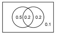
$\Rightarrow \quad \frac{P(A \cap B)}{P\left(A \cup B^C\right)}=\frac{0.2}{0.5+0.2+0.1}=\frac{2}{8}=\frac{1}{4}$
Hence, the correct answer is $\frac{1}{4}$.

Question 3: The probability of forming a 12-person committee from 4 engineers, 2 doctors, and 10 professors containing at least 3 engineers and at least 1 doctor is:

Solution:
3 engineering + 1 doctor + 8 Professors $\rightarrow{ }^4 \mathrm{C}_3 \cdot{ }^2 \mathrm{C}_1 \cdot{ }^{10} \mathrm{C}_8$ $=360$
3 engineering +2 doctors +7 Professors $\rightarrow{ }^4 \mathrm{C}_3$. ${ }^2 \mathrm{C}_2 \cdot{ }^{10} \mathrm{C}_7$ $=480$
4 engineering +1 doctor +7 Professors $\rightarrow{ }^4 \mathrm{C}_4 \cdot{ }^2 \mathrm{C}_1 \cdot{ }^{10} \mathrm{C}_7$ $=240$
4 engineering +2 doctors +6 Professors $\rightarrow{ }^4 \mathrm{C}_4$. ${ }^2 \mathrm{C}_2 \cdot{ }^{10} \mathrm{C}_6$ $=210$
Total $=1290$
Required probability $=\frac{1290}{{ }^{16} \mathrm{C}_{12}}$
$=\frac{1290}{1820}$
$=\frac{129}{182}$
Hence, the correct answer is $\frac{129}{182}$.

NCERT Class 12 Maths Notes – Chapter-Wise Links

For students' preparation, Careers360 has gathered all Class 12 Maths NCERT notes here for quick and convenient access.

Subject-Wise NCERT Exemplar Solutions

After finishing the textbook exercises, students can use the following links to check the NCERT exemplar solutions for a better understanding of the concepts.

• NCERT Exemplar Class 12 Solutions

• NCERT Exemplar Class 12 Maths

• NCERT Exemplar Class 12 Physics

• NCERT Exemplar Class 12 Chemistry

• NCERT Exemplar Class 12 Biology

Subject-Wise NCERT Solutions

Students can also check these well-structured subject-wise solutions.

• NCERT Solutions for Class 12 Mathematics

• NCERT Solutions for Class 12 Chemistry

• NCERT Solutions for Class 12 Physics

• NCERT Solutions for Class 12 Biology

NCERT Books and Syllabus

Students should always analyse the latest syllabus before making a study routine. The following links will help them check the syllabus. Also, give them access to some reference books.

• NCERT Books Class 12 Maths
• NCERT Syllabus Class 12 Maths
• NCERT Books Class 12
• NCERT Syllabus Class 12