Applications Of Differentiation In Mechanics: Velocity And Acceleration

Mechanics is like the superhero of physics that helps us understand how things move and why. And guess what? Differentiation, which sounds like a big and fancy, even scary word, is like a magic tool in mechanics. It helps us figure out how things are speeding up, slowing down, and changing directions.

What Is Differentiation?

Let's quickly understand differentiation. Imagine you're on a road trip, and you want to know how fast you're going. You look at your speedometer, and it tells you the speed at that very moment. Now, if you want to know how your speed changes over time, that's where differentiation comes in. It's like asking, "Hey, how much is my speed changing every second?"

Velocity: How Fast and In Which Way?

Let's talk about velocity. When you're driving your car, you want to know not only how fast you're going but also in which direction. Velocity gives you both of these things. It's like a super detailed speed that tells you if you're going forward, backward, left, or right.

Now, let's use differentiation to understand this better. Imagine you're riding a bicycle, and you're tracking your position over time. If you take the derivative of this position function, you get the velocity function. This function shows you how fast you're pedalling at any given moment.

For instance, if you're tracking your position with the function s(t) = 2t² + 3t, where s is your position and t is time, the derivative s'(t) will give you the velocity. It will show you how quickly your position is changing at any time.

Also Read - Understanding The Maths Behind Faraday's Law Of Electromagnetic Induction

Acceleration: Changes In Speed

Now, let's talk about acceleration. This is like the superhero sidekick of velocity. While velocity tells you how fast you're going, acceleration tells you how much you're speeding up or slowing down.

Here's where differentiation comes to the rescue again. If you take the derivative of the velocity function, you get the acceleration function. This function tells you how much your velocity is changing at each moment.

Imagine you're in a car, and you step on the gas pedal. Your speed goes from 0 to 60 mph in a few seconds. That's acceleration at work. If your velocity is changing a lot, you have high acceleration. If your velocity is changing just a little, you have low acceleration.

These concepts find their home in the CBSE Class 11 in the chapter titled "Motion in a Straight Line." Here, you'll unravel the concepts of velocity and acceleration in their theoretical context. This chapter forms the foundation for your understanding of how objects move and how their velocity changes over time.

As you venture into the competitive exam arena, like JEE, NEET, CBSE, and other Board exams, a good command of applications of differentiation becomes a powerful tool. Mechanics questions often involve calculating velocities, predicting accelerations, and analysing motion patterns. Differentiation equips you with the mathematical tools to excel in these questions, helping you score higher and stand out among the crowd.

Derivatives In Mathematics

Here are a few cases that demonstrate how derivatives are super useful in the real world of mathematics:

Rate Of Change Of A Quantity

One of the most essential applications of derivatives is to determine the rate of change of a quantity. For instance, when analysing the volume of a cube as its sides decrease, the derivative helps find how the volume changes concerning the sides' variations.

Increasing And Decreasing Functions

Derivatives aid in identifying whether a function is increasing, decreasing, or constant. By analysing the sign of the derivative within a given interval, we can ascertain the behaviour of the function in that range.

If you have a function f that's continuous between p and q and differentiable within that open interval, here's how it behaves:

• If f'(x) is greater than zero for each x in the range (p, q), then f is increasing from p to q.

• If f'(x) is less than zero for each x in the range (p, q), then f is decreasing from p to q.

• If f'(x) equals zero for each x in the range (p, q), then f is a constant function from p to q.

Tangent And Normal To A Curve

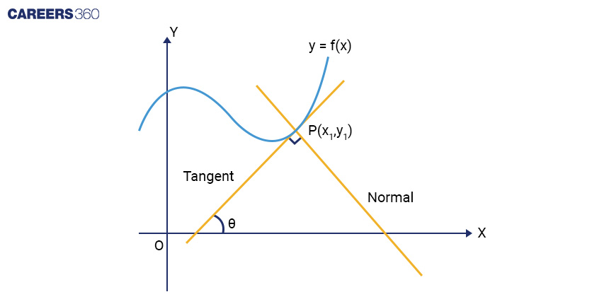
Derivatives play a crucial role in understanding the behaviour of curves. The slope of the tangent to a curve at a specific point is given by the derivative at that point. Similarly, the normal to the curve, which is perpendicular to the tangent, can be expressed in terms of the derivative.

Imagine the tangent line connecting with the curve at the point P (x₁, y₁).

Also Read - Differential Equations In Electromagnetism: Solving Problems With Calculus

Now, if we consider a straight line passing through a point and having a slope denoted as m, its equation can be represented as:

y – y₁ = m(x – x₁)

From the equation above, we can observe that the slope of the tangent to the curve y = f(x) at the point P(x₁, y₁) is represented by the derivative dy/dx at that point, which can be denoted as f'(x). Therefore,

The equation of the tangent line to the curve at the point P(x₁, y₁) can be expressed as:

y – y₁ = f'(x₁)(x – x₁)

Similarly, the equation of the normal line to the curve can be determined using the following expression:

y – y₁ = [-1/ f '(x₁)] (x – x₁)

Alternatively, this can be written as:

(y – y₁) f'(x₁) + (x - x₁) = 0

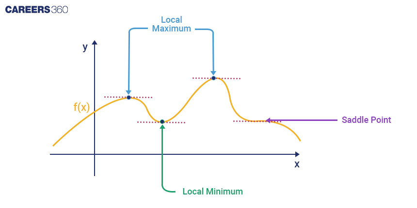
Maxima And Minima

Derivatives help identify the highest and lowest points of a curve, known as maxima and minima, respectively. These points hold significance in various optimization problems and are crucial for determining turning points in a function.

• When x = a, if f(x) is less than or equal to f(a) for all x in its domain, then f(x) has an Absolute Maximum value at a.

• When x = a, if f(x) is less than or equal to f(a) for all x in an open interval (p, q), then f(x) has a Relative Maximum value at a.

• When x = a, if f(x) is greater than or equal to f(a) for all x in its domain, then f(x) has an Absolute Minimum value at a.

• When x = a, if f(x) is greater than or equal to f(a) for all x in an open interval (p, q), then f(x) has a Relative Minimum value at a.

Monotonicity

Derivatives contribute to determining whether a function is monotonic, meaning it is either consistently increasing or decreasing across its entire domain. This concept is vital in understanding the behaviour of functions and their trends.

For small positive h, if f(x + h) < f(a), then the function is monotonically decreasing at x = a.

• If the function increases, its derivative f'(x) is positive.

• If the function decreases, its derivative f'(x) is negative.

• At points of maximum or minimum, its derivative f'(x) is zero.

Approximation

Derivatives can be used to provide approximate values for small changes or variations in a quantity. This is particularly useful when precise values are difficult to obtain.

Imagine a shift in the x value, denoted as dx, is equivalent to the value of x itself.

So, the rate of change dy/dx becomes like a small change Δx, which is basically x.

Because this change dx is nearly the same as x, it means that dy is approximately equal to y

Point Of Inflection

When dealing with a continuous function f(x), a point x0 is referred to as an "inflection point" under the following conditions: if f'(x0) = 0 or the second derivative f’’(x0) doesn't exist where f '(x0) does, and if the sign of f ’’(x) changes as it goes through x = x0.

• If f’’(x) < 0 for x ∈ (a, b), then the curve represented by y = f(x) is curving downward, which is called "concave downward."

• Conversely, if f’’(x) > 0 for x ∈ (a, b), then the curve y = f(x) is curving upward, known as "concave upwards" in the interval (a, b).

For instance, consider the function f(x) = sin x:

Solution:

The first derivative is f'(x) = cos x. The second derivative is f’’(x) = -sin x. At points where sin x = 0 (for instance, when x = nπ, where n is an integer), the curve's concavity changes.

Chandrayaan 3: Helping In Gentle Lunar Touchdown

Advancements in space missions showcase how differentiation concepts shape groundbreaking developments. Chandrayaan 3, the lunar mission by ISRO, embarked on a journey to explore the Moon's mysteries. The delicate task of landing on the lunar surface required meticulous calculations of velocity and acceleration. By utilising differentiation, scientists could precisely compute the instantaneous velocity of the spacecraft and adjust acceleration patterns, ensuring a soft landing. This successful endeavour demonstrates how mathematical tools like differentiation transform into real-world achievements, paving the way for scientific exploration.

Also Read - Mathematics In Aviation: Analysing Flight Trajectories

Solved Problems

Imagine a racing car accelerating along a straight track. The car's position function is given by s(t) = 4t² + 3t + 1, where s is in metres and t is in seconds. Calculate the car's instantaneous velocity at t = 2 seconds using differentiation.

Solution:

Instantaneous velocity is the derivative of the position function with respect to time, v(t) = ds/dt.

Given s(t) = 4t² + 3t + 1,

Differentiate s with respect to t: v(t) = d/dt (4t² + 3t + 1)

= 8t + 3.

Substitute t = 2 seconds: v(2) = 8(2) + 3

= 16 + 3

= 19 m/s.

So, at t = 2 seconds, the car's instantaneous velocity is 19 m/s.

Hope you have now gained a comprehensive understanding of the differentiation and its applications during the exams and everyday life.